Evaluating Model-Agnostic Prediction Intervals: The Case of nnetsauce's QuantileRegressor

When you think about model predictions, what's often overlooked is the level of confidence in these forecasts. Point predictions might tell you what's expected, but they leave you guessing about the reliability of those figures. This uncertainty can lead to substantial variations in decision-making processes, particularly in critical fields such as finance, healthcare, and policy-making.

The nnetsauce library's QuantileRegressor attempts a different approach. Rather than providing just a single method to generate prediction intervals, it incorporates a variety of model types. Any model that supports .fit() and .predict(), including simple linear regressors, support vector regression, or even complex random forests, can morph into a quantile forecasting tool. This transformation hinges on optimizing an offset around point predictions to minimize the pinball (or quantile) loss. In practice, this means QuantileRegressor provides a flexible framework that adapts to the strengths of the underlying models it employs, rather than forcing a one-size-fits-all solution. The flexibility extends to five scoring strategies that define how this offset is calculated: predictions, residuals, conformal, studentized, and conformal-studentized.

Availability of the Library in Python and R

In addition to Python, this functionality is also present in R through nnetsauce_r. Importantly, this isn't just a different version; it's a lightweight reticulate wrapper around the original Python module. This design choice means that R users can access the full capabilities of nnetsauce while maintaining simplicity. So when you audit the behavior in R, you’re actually examining the Python source directly, simplifying the verification process for users who work in both environments. The move to bridge these ecosystems certainly caters to a growing demographic of analysts who rely on both programming languages.

For Python users, below is a sample implementation that demonstrates its practical use:

from nnetsauce.quantile.quantileregression import QuantileRegressor
model = QuantileRegressor(
    obj=BayesianRidge(),  # integrates with any sklearn-compatible regressor
    level=95,  # desired coverage percentage
    scoring="residuals",  # choose from several scoring methods
)
model.fit(X_train, y_train)
result = model.predict(X_test, return_pi=True)
# result contains mean, lower, median, and upper bounds

For R users, the implementation is equally straightforward, utilizing the same Python class as outlined above:

library(datasets)
X <- as.matrix(mtcars[, -1]); y <- mtcars[, 1]
sklearn <- nnetsauce::get_sklearn()
model <- sklearn$linear_model$BayesianRidge()
quantile_model <- QuantileRegressor(model, level = 95, scoring = "residuals")
quantile_model$fit(X_train, y_train)
print(quantile_model$score(X_test, y_test))

Ready to get started? Let’s look into installing the library and running through the quickstart guide.

# To install the nnetsauce library, run:
import sys, subprocess
subprocess.run([sys.executable, "-m", "pip", "install", "-q", "nnetsauce", 
"--break-system-packages"], check=False)
import warnings
warnings.filterwarnings("ignore")
from nnetsauce.quantile.quantileregression import QuantileRegressor
from nnetsauce.predictioninterval.predictioninterval import PredictionInterval
from sklearn.linear_model import BayesianRidge
from sklearn.datasets import load_diabetes
from sklearn.model_selection import train_test_split
import numpy as np

# Load the diabetes dataset and prepare for training
X, y = load_diabetes(return_X_y=True)
X_train, X_test, y_train, y_test = train_test_split(X, y, test_size=0.3, random_state=42)
model = QuantileRegressor(obj=BayesianRidge(), level=95, scoring="residuals")
model.fit(X_train, y_train)
result = model.predict(X_test, return_pi=True)
coverage = np.mean((y_test >= result.lower) & (y_test <= result.upper))
print("First 5 intervals:")
for lo, med, hi, true in zip(result.lower, result.median, result.upper, y_test)[:5]:
    print(f" [{lo:7.1f}, {hi:7.1f}] median={med:7.1f} true={true:7.1f}")
print(f"\nEmpirical coverage on the test set: {coverage:.1%} (target: 95%)")
First 5 intervals:
[ 35.9, 243.1] median= 137.3 true= 219.0
[ 76.6, 283.8] median= 177.9 true= 70.0
[ 27.8, 235.0] median= 129.2 true= 202.0
[ 186.7, 394.0] median= 288.1 true= 230.0
[ 18.6, 225.8] median= 119.9 true= 111.0
Empirical coverage on the test set: 94.7% (target: 95%)

Testing the Capabilities

For the evaluation, I conducted a comprehensive grid search without any hyperparameter tuning. The goal was to observe the wrapper's effects in its natural state, akin to how a first-time user would implement it. This decision is significant because it helps to demonstrate how the QuantileRegressor performs out of the box, which is often when users will rely on it most heavily:

• 38 scikit-learn regressors were employed, covering everything returned by sklearn.utils.all_estimators(type_filter='regressor'), with the exception of meta-estimators requiring additional configuration.
• 6 datasets were tested: diabetes, linnerud, two synthetic datasets, an anonymized version of the classic Boston Housing dataset, and a subset of California Housing data.
• 2 coverage targets were evaluated: 80% and 95%.
• 5 scoring methods were available for QuantileRegressor, in addition to the sibling class PredictionInterval with a different structural baseline.
• Two direct quantile methods were referenced: scikit-learn’s built-in linear QuantileRegressor (using pinball loss minimization) and GradientBoostingRegressor(loss="quantile") that operates independently without wrapping another model.

This means conducting 2,736 model fits for the wrapped regressors plus an additional 24 for the native baselines. The sheer scale of this test reflects an understanding that quantile regression can be sensitive to the choice of both models and data characteristics. Results need significant contextualization, and there’s a lot to unpack in terms of performance metrics, coverage accuracy, and overall predictive power.

# Importing necessary libraries and establishing metrics
import time
import numpy as np
import pandas as pd
from collections import namedtuple
from sklearn.base import BaseEstimator, RegressorMixin, clone
from sklearn.utils import all_estimators
from sklearn.model_selection import train_test_split
from sklearn.datasets import load_diabetes, load_linnerud, make_regression
from scipy.optimize import differential_evolution
import matplotlib.pyplot as plt

np.random.seed(42)
LEVELS = [80, 95]
SCORINGS = ["predictions", "residuals", "conformal", "studentized", "conformal-studentized"]

def coverage_and_width(y_true, lower, upper):
    covered = (y_true >= lower) & (y_true <= upper)
    return covered.mean(), np.mean(upper - lower)

print("Metrics ready.")
# Preparing datasets for a comprehensive grip on the results
import urllib.request, io
def load_datasets():
    datasets = {}
    X, y = load_diabetes(return_X_y=True)
    datasets["diabetes"] = (X, y)
    lin = load_linnerud()
    datasets["linnerud (predict weight)"] = (lin.data, lin.target[:, 0])
    return datasets

DATASETS = load_datasets()
for name, (X, y) in DATASETS.items():
    print(f"{name:45s} X={X.shape} y={y.shape}")
diabetes X=(442, 10) y=(442,)
linnerud (predict weight) X=(20, 3) y=(20,)

Key Findings: Reliability Under Evaluation

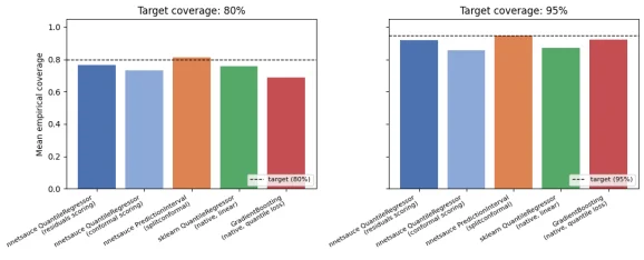
After filtering out the runs that encountered issues, it’s critical to understand how often the median coverage from QuantileRegressor fell within a mere three percentage points of the target level. This comparison becomes even more interesting when set against the native baselines. Was it consistent? What other factors influenced these results? Let's explore that further.

During the testing, several factors emerged that could sway performance results. These include the choice of base estimator, the dataset characteristics, and, importantly, the scoring methods utilized. For instance, using residuals as the scoring method often revealed insights that other methods overlooked, providing a clearer picture of model performance across different cases. This nuanced analysis is essential because it brings to light how models can produce varying results under slight modifications in methodology, leading to substantial implications for practitioners in the field.

Future Outlook: Awareness and Adaptation

If you're working in this space, the take-home message should be clear: the framework surrounding quantile regression must be chosen with care. It isn’t just about picking the latest or the most popular tool; it’s about understanding the intricacies of your data and how different models respond to it. What stands out to me is the growing emphasis on robust statistical principles in prediction interval generation.

The analysis presented here shines a spotlight on the growing importance of selecting the right estimation technique for generating reliable prediction intervals. With models like `PredictionInterval` demonstrating superior calibration compared to even the traditional methods, there's an emerging framework for tackling uncertainties in regression tasks. It’s vital to keep abreast of developments in the field, including hybrid models that blend the strengths of traditional techniques with modern adaptive methods. Trust me, this is more significant than it looks. The appetite for robust statistical models capable of addressing uncertainties will only deepen, pushing the boundaries of what we once thought was possible in model accuracy and reliability.

People often overlook a critical point: while an average performance might be satisfactory, it’s the edge cases that frequently reveal weaknesses in a model. Those working on real-world datasets should always validate predictions rigorously. Running coverage checks on your unique datasets remains a non-negotiable step to ensure accuracy, because relying solely on general performance metrics won’t cut it.